Part 2: Using appropriate mathematical and physiological analyses shows that Stryd power is strongly correlated to metabolic rate across speed

Note: Independent academic research helps to drive innovation. At Stryd, we are researchers, first and foremost. It’s always exciting to us to read about and learn from new testing of sports technology innovations by the wider research community. However, we are responding in detail now to research that we believe needs correcting regarding proper mathematical and physiological analyses. Science is self-correcting, and we believe that taking this opportunity to respond is an important and integral part of the evolution of sports technology.

Please read the post below. We encourage you to join in the discussion.

• Part 1: New Research Data Shows Stryd Pioneer Power Correlates with Metabolic Expenditure (June 2018)
• Part 2: Using appropriate mathematical and physiological analyses in Aubry et al. 2018 (December 2018)
• Part 3: Replying to the Response to Our Manuscript Clarification of Aubry et al. 2018 (December 2018)

Earlier this year, Aubry et al. published a paper using Stryd Pioneer entitled “An assessment of running power as a training metric for elite and recreational runners” (Aubry et al., 2018).

Manuscript Clarification: Methodological Flaws in Aubry, RL, Power, GA, and Burr, JF. An Assessment of Running Power as a Training Metric for Elite and Recreational Runners (December 2018)

Author Response to the Manuscript Clarification: Author Response (December 2018)

In the study, the authors collected data for elite and recreational runners across speeds and surfaces. They then compared Stryd power values divided by speed to rate of oxygen consumption values divided by speed, pointing out that these values were not strongly correlated. They subsequently came to the conclusion "Running power is not sufficiently accurate as a surrogate of metabolic demand." This message then was tweeted by the authors and shared widely, without the methods behind that result being thoroughly checked. While we agree that Stryd does not account for every minor influence on rate of oxygen consumption, the overall conclusion of the article is incorrect, largely due to dividing these two values by speed before comparing them. We show this using the following analogy and analysis of real data.

The purpose of this blog post is to point out the biggest methodological flaw in the paper, and to use every day analogies and real data to show how this analysis error led to the false conclusion stated in the paper. We discuss the other major flaw, which, though less serious, still could have a large effect on conclusions in another blog post. This post can be found here.

Analogy: Food and Housing Expenditure Across Income

Consider the following analogy. Like both the Stryd power values and rate of oxygen consumption are dependent upon on speed, both housing and food budget are dependent upon a person’s income. The more income a person earns, the more they will pay for housing. For the sake of this example we will assume this relationship is approximately linear. *

Even though having no income whatsoever would imply no money for housing, we did add a small positive intercept ($6000), to show that our example holds even for small, non-zero intercept values. We are assuming housing to be approximately 30% of total income. Noise is added to the system via a uniform distribution with a mean of 0 and a range of -$1500 to $1500.

* Note: this example is for explanation purposes only. We looked up all of these data for American incomes, and as income increases, the percentage spent on necessities actually decreases because people save more money for retirement and spend a larger percentage of income on non-necessities. It is an excellent commentary on the effects of income inequality on long-term fiscal prospects, but not particularly helpful for the purposes of this explanation. For a graphical depiction of these patterns, see this webpage.

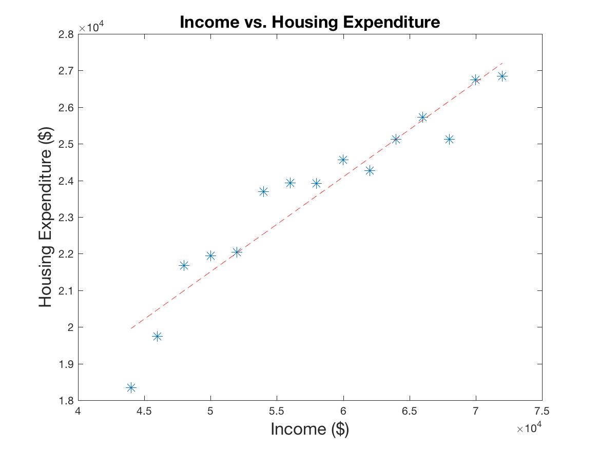
Figure 1a: Income vs. Housing Expenditure. The line shows the best linear fit to the data: R=0.95.

A similar relationship occurs with food expenditure. The more a person earns in income, the more money they have available to pay for food. Again, we model this relationship to be linear, with a small magnitude y-intercept. We are assuming food to be approximately 12% of total income. Noise is added to the system via a uniform distribution with a mean of 0 and a range of -$500 to $500.

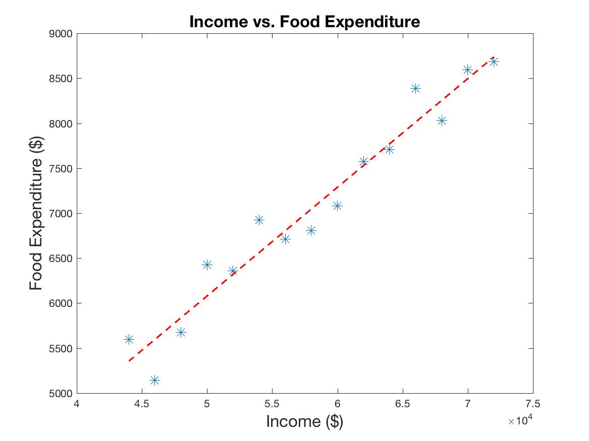
Figure 1b: Income vs. Food Expenditure. The line again shows the best linear fit to the data: R=0.97.

Now, since both housing and food budgets are linearly dependent upon income, graphing the one vs. the other also leads to a strongly linear relationship.

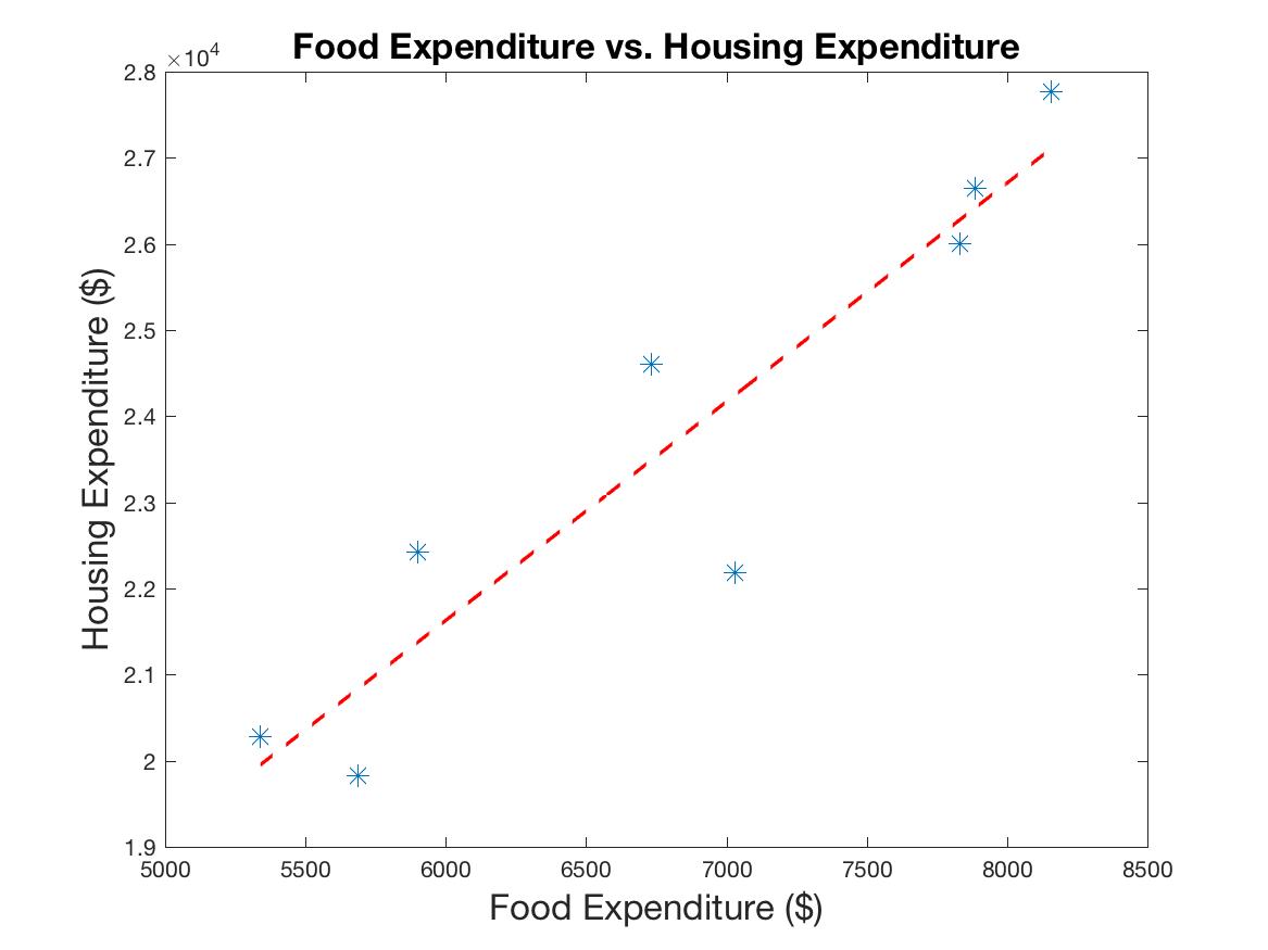
Figure 2a: Food vs. Housing Expenditure. The line shows the best linear fit to the data: R=0.94.

However, when each of these variables is normalized by income, the relationship disappears. By dividing by income, the dependence of each of these variables on income was eliminated, therefore destroying their strong relation with each other. The reason this occurs in this particular example is because there is an approximately proportional relationship of the variables with income, or approximately a zero intercept. Therefore, dividing by income gives approximately a constant value for each. We thus get a cloud of points indicative of the variability across samples due to noise rather than a linear relationship. The actual percentages are not quite right because of both noise and a non-zero intercept, but there is no linear relationship in the normalized data.

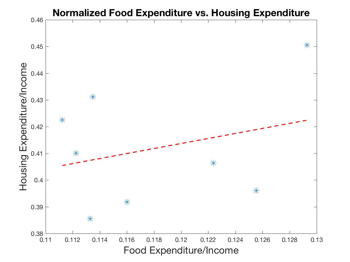
Figure 2b: Food vs. Housing Expenditure, normalized by income. There is virtually no meaningful correlation between the data: R=0.07.

Appropriate Analysis of Available Data.

An analogous situation occurs with the data graphed in Figure 1 of the authors’ paper (Aubry et al., 2018). Rate of oxygen consumption is approximately proportional to speed (linearly dependent upon speed with a y-intercept of close to zero) across both elite and recreational runners (Batliner et al., 2018). This means all values for the rate of oxygen consumption measure when normalized by speed (otherwise known as cost of transport)* will be approximately constant, giving virtually no variation in these values other than that due to noise or subject variation. Therefore, regardless of Stryd power’s dependence upon speed, no correlation would be expected between the normalized measures. Stryd power’s strong linear correlation with rate of oxygen consumption, however, indicates increasing Stryd power with increasing speed, meaning any variability would be reduced by normalization with speed. Thus, any correlation whatsoever between the normalized measures would be small and due to chance, unaccounted for nonlinearities, or subject variation, not the dominant linear relation with speed that underlies both non-normalized measures.

* Note: The authors use the term “metabolic demand” to refer to both “rate of oxygen consumption,” which is the oxygen consumption over a given period of time, and for “metabolic cost,” often called “cost of transport,” which is oxygen consumption per unit distance. These are fundamentally different measures and consequently have fundamentally different relationships with speed. Namely, cost of transport in running has long been known not to vary significantly across speed (Margaria et al., 1963).

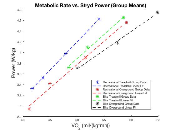
Figure 3a: Group mean data and best linear fits the group means for recreational and elite runners overground and on a treadmill. All individual fits had R>0.99.

Because we were unable to obtain the individual subject data from the authors, we instead simulated the effect of having multiple subjects by adding variability by combining the data sets across subject groups and conditions. Note that this variability may be greater due to the methodological discrepancies with rate of oxygen consumption data collection on the treadmill vs. overground, as discussed in our other blog post. Specifically, rate of oxygen consumption over rougher terrain is already 10% larger than flat surface data (Gantz and Derrick, 2018). If the treadmill data were not at steady-state, but underestimated due to the trials being too short, this difference would be still larger. We pooled all of the rate of oxygen consumption and Stryd power data presented in Table 2 together into one large data set and performed a linear fit on these data.

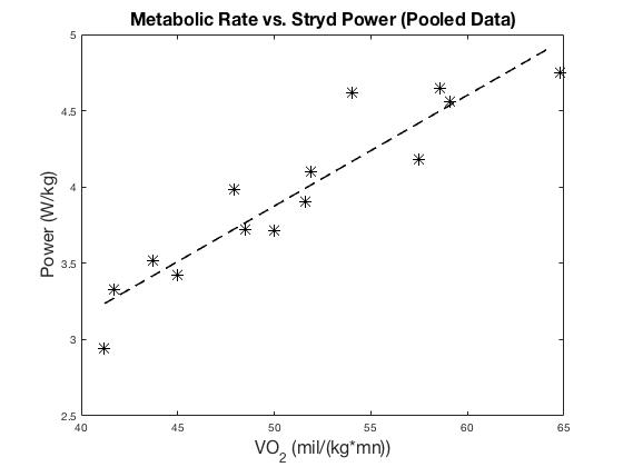
Figure 3b: Pooled group mean data across subject populations and conditions, providing reasonable variability, and the best linear fit. R=0.93.

It is important to note that, though we performed this analysis on multiple data points in order to get a lower bound on the correlation value, Stryd power data are tailored to the individual, with power calculations being performed using input data for each specific subject, not across subjects. Therefore, if one were to actually validate Stryd power’s values as a training metric, as the paper’s title implies, correlation coefficients between rate of oxygen consumption and Stryd power should only be performed on a subject-by-subject basis. For those who have a statistical objection to performing the correlation analysis this way, we completely understand your objections. Please see the supplemental statistical section at the end of the blog for clarification as to why this instance is different than in typical calculations of correlation values and how one would inject variability into the data in a statistically and functionally meaningful way.

Clearly, even with variability across groups and conditions introduced into the relation, there is still a very strong linear relationship between the rate of oxygen consumption values and the Stryd power values.

This strong dependence is obviously significantly reduced when these values are normalized by speed, giving a value only slightly larger than that found in the paper.

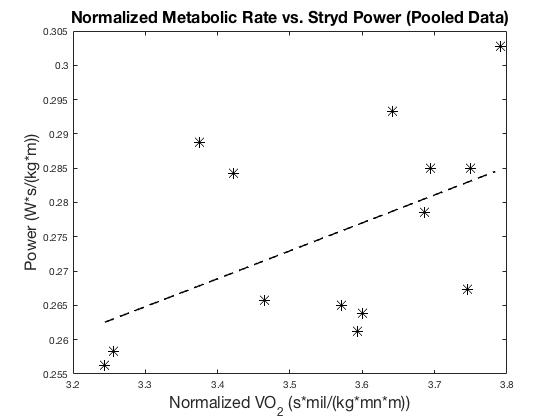
Figure 3c: Pooled group mean data normalized by speed across subject populations and conditions, providing reasonable variability, and the best linear fit. R=0.50. We used similar units to be consistent with Figure 2 of (Aubry et al., 2018).

To do a proper statistical analysis of non-normalized, non-averaged data collected using consistent data collection methods, we used individual rate of oxygen consumption and Stryd power data we had previously collected on 10 subjects across a range of velocities using the Stryd Pioneer used in the paper. We used an increasing speed, ramp-up protocol with a minimum of 4 minutes per trial, but additionally examined slope to determine that all subjects had reached steady state for all metabolic data used in analysis. We then fit these data both on a subject-by-subject basis, as Stryd is designed to be used, and then using the pooled individual data, to again provide a lower bound for a correlation coefficient. We used both the proper, non-normalized measures (Figure 4a), and the measures normalized by speed, as was performed in the paper (Figure 4b).

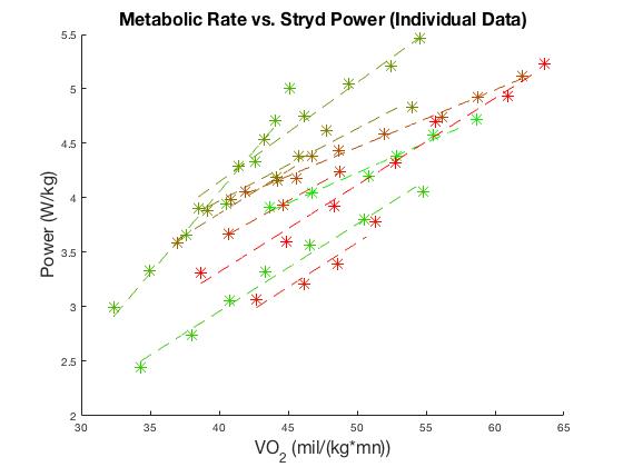
Figure 4a: Rate of oxygen consumption vs. Stryd data for 10 subjects across speed with linear fits. R values ranged from 0.96 to 0.99, with a mean of 0.99.

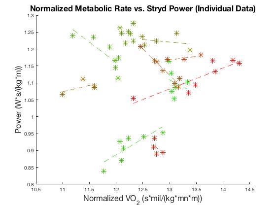
Figure 4b: Rate of oxygen consumption vs. Stryd data normalized by speed for 10 subjects across speed with linear fits. R values ranged from 0.04-0.97 with a mean of 0.6. We used similar units to be consistent with Figure 2 of (Aubry et al., 2018).

Clearly, the data show that, when not grouped together, the Stryd power and rate of oxygen consumption data are tightly, linearly coupled with high correlation coefficients.

We then pooled the data across all subjects to perform an analysis to determine a lower bound on the correlation coefficient for the data.

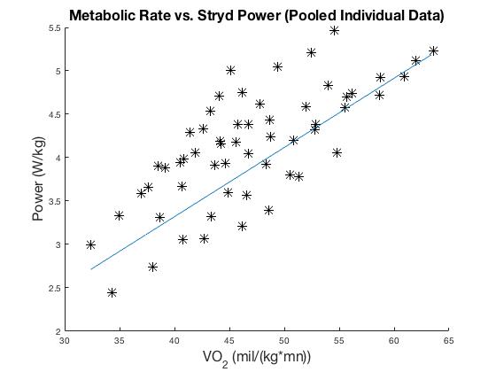
Figure 4c: Rate of oxygen consumption vs. Stryd data for pooled data from 10 subjects across speed with a linear fit. The correlation coefficient R value was 0.73.

Finally, we normalized the pooled data, to give a figure equivalent to Figure 2 in the paper for our data. We very clearly see a non-significant R value for this relationship.

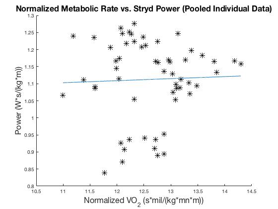
Figure 4d: We took pooled data from 10 subjects and normalized both rate of oxygen consumption and Stryd power values by speed. The linear fit of the resulting data gave an R value of 0.04. We used similar units to be consistent with Figure 2 of (Aubry et al., 2018).

Why the discrepancy between Figures 4c and 4d? Both Stryd power and rate of oxygen consumption have linear relationships with speed, but with close to zero intercepts. Therefore, these linear relationships are negated by normalization by speed. We then get a cloud of points, and the correlation between rate of oxygen consumption and Stryd power output also disappears.

In conclusion, it is obvious from the comparison of the analogy data, the data we analyzed from Table 2 in (Aubry et al., 2018) and both our appropriate analyses and our repetition of the methods used in the paper on our own data that there is a clear, linear relationship between oxygen consumption and Stryd’s power measure. Further analysis shows that this relationship results from the linear relationship between speed and rate of oxygen consumption, and the linear relationship between speed and power. Normalization by speed negates each of these linear dependencies due to their small intercepts, leading to the expected lack of correlation between “metabolic demand” (actually cost of transport) and normalized power found by the authors.

Again, what the authors call normalized metabolic demand is actually cost of transport. Cost of transport varies little across speed (Margaria et al., 1963, Bramble and Lieberman, 2004). Steudel-Numbers and Wall-Scheffler found shallow parabolic relationships within subjects, but no linear variation (Steudel-Numbers and Wall-Scheffler, 2009). Therefore, no linear relationship would be expected with the Stryd data because very little if any variability is expected in the cost of transport values. Expecting cost of transport to change across speed in running would be like expecting percentage of income spent on food to change across income level in our earlier example.

Statistical Notes (written by Dr. Kristine L. Snyder)

How to properly aggregate your data for correlation analysis depends upon what you are trying to determine. The purpose of the paper as stated is to assess the use of power as a training metric, and its conclusion is that power is not a sufficient surrogate for metabolic cost. However, this paper aggregates data across subjects and then correlates, whereas our training metrics are tailored to the individual, use their anatomical data as inputs, and should only be tested on an individual basis.

Take my husband and I for example. I’m very economical across running speed. I have virtually no engine to speak of (low VO2 max), but I am really economical, so have a low metabolic rate for a given speed, kind of like a Prius. My husband, on the other hand, is not economical, but has a great engine (VO2 max), kind of like a Porsche. (He will deny this; don’t believe him because he sells himself short.) His metabolic rate values for a given speed on the level are much higher than mine. Even if using my Stryd power data gives really accurate metabolic rate estimates for my data, it won’t give accurate estimates for his. However, I’m never going to use his Stryd device. I’m going to use mine, with algorithms that are tailored to my input data. His Stryd won’t work well for me any more than his shoes will. All that matters in terms of assessment of Stryd as a training metric is how well my device works for me and his works for him, even if our linear relationships between Stryd power and metabolic rate have completely different parameters. Aggregating our data and analyzing whether the same linear relationship works for both our data does not actually assess how Stryd is used in practice.

Statistically speaking, in order to add the proper variability into the data and to have a better data point to parameter ratio, what everyone collecting these data should really do is to take multiple data points for metabolic rate and Stryd power for each subject at many speeds and include them all in the analysis. Our metabolic rate at a given speed is not always consistent across trials. However, we don’t have these data for Stryd Pioneer. It’s an outdated device. There is no reason for us to go back and collect data with a device we do not use anymore when we have built a better one. I have talked to the rest of the Stryd team about this, and we will be using this method for future validation studies.

About the Author

Dr. Kristine L. Snyder earned her bachelor’s degree magna cum laude in Mathematics and Physics at Bryn Mawr College, where she also ran cross-country and indoor and outdoor track. She did her first master’s on the biomechanics and physiology of running with Prof. Claire Farley in University of Colorado’s Integrative Physiology Department. She then got a master’s and PhD in Applied Mathematics from University of Colorado, where her dissertation work was co-advised by Prof. Rodger Kram in Integrative Physiology. She worked on system identification of temporal dynamics of metabolic minimization with Prof. Max Donelan (Simon Fraser), elastic energy storage and return uphill and downhill running with Prof. Jinger Gottschall (Penn State), and algorithmic development for discrete mechanics for optimal control with Prof. Todd Murphey (Northwestern), among other projects. During her time at CU, she taught and TA’d courses such as undergraduate and graduate statistics, biomechanics, all levels of calculus, and differential equations. She received an NSF postdoctoral fellowship in biology to work with Prof. Dan Ferris, then at University of Michigan, now at University of Florida, on connectivity during locomotor activities, during which she started a neuroscience camp for middle and high school girls. She recently left a tenure-track position in Mathematics and Statistics at University of Minnesota Duluth where she was a 3rd generation professor after three years. She moved back to Boulder to take a position at Stryd that allows her to use all of her degrees to better runners’ experiences and performances. Her publications are available on ResearchGate.

References

AUBRY, R. L., POWER, G. A. & BURR, J. F. 2018. An assessment of running power as a training metric for elite and recreational runners. J Strength Cond Res, 32, 2258-2264.
BATLINER, M. E., KIPP, S., GRABOWSKI, A. M., KRAM, R. & BYRNES, W. C. 2018. Does metabolic rate increase linearly with running speed in all distance runners? Sports Medicine International Open, 2, E1-E8.
BRAMBLE, D. M. & LIEBERMAN, D. E. 2004. Endurance running and the evolution of Homo. Nature, 432, 345-52.
GANTZ, A. M. & DERRICK, T. R. 2018. Kinematics and metabolic cost of running on an irregular treadmill surface. J Sports Sci, 36, 1103-1110.
MARGARIA, R., CERRETELLI, P., AGHEMO, P. & SASSI, G. 1963. Energy cost of running. 18, 367-370.
STEUDEL-NUMBERS, K. L. & WALL-SCHEFFLER, C. M. 2009. Optimal running speed and the evolution of hominin hunting strategies. Journal of Human Evolution, 56, 355-360.